38


                Geotechnical News • December 2012


                www.geotechnicalnews.com


                GROUNDWATER


              errors once a finite element solution
            
            
              has been obtained. The procedure
            
            
              is referred to “adaptive” since the
            
            
              process depends on previous results at
            
            
              all stages.
            
            
              Various procedures exist for the
            
            
              refinement of finite element solutions.
            
            
              Broadly these fall into two categories
            
            
              (Zienkiewicz et al., 2005).
            
            
              1. The


                h


              -refinement in which the same
            
            
              class of element continues to be
            
            
              used but it is changed in size, in
            
            
              some locations while being made
            
            
              larger in some locations and small-
            
            
              er in others, to provide maximum
            
            
              economy in reaching the desired
            
            
              solution,
            
            
              2. The


                p


              -refinement in which the same
            
            
              element size is used and there is a
            
            
              simple increase, generally hierar-
            
            
              chically, in the order of polynomial
            
            
              used in the definition of the ele-
            
            
              ments.
            
            
              It is occasionally useful to divide the
            
            
              above categories into subclasses, as
            
            
              the


                h-


              refinement can be applied and
            
            
              thought of in different ways. Three
            
            
              typical methods of


                h


              -refinement are:
            
            
              1. Element subdivision – if existing el-
            
            
              ement show too large an estimated
            
            
              error, the elements are simply di-
            
            
              vided into smaller elements while
            
            
              keeping the original element geom-
            
            
              etry boundaries intact,
            
            
              2. Mesh regeneration (remeshing) – on
            
            
              the basis of a given solution, a new
            
            
              element size is predicted in all the
            
            
              domains and a totally new mesh is
            
            
              generated,


                3. r


              -refinement – keeps the total num-
            
            
              ber of nodes constant and adjusts
            
            
              their position to obtain an optimal
            
            
              approximation. This method is dif-
            
            
              ficult to use in practice and there is
            
            
              little reason to recommend its us-
            
            
              age.
            
            
              The


                p


              -refinement subclasses are:
            
            
              1. one in which the polynomial order
            
            
              is increased uniformly throughout
            
            
              the entire domain,
            
            
              2. one in which the polynomial order
            
            
              is increased locally while using hi-
            
            
              erarchical refinement.
            
            
              Occasionally it is efficient to combine
            
            
              the


                h


              - and


                p


              - refinements and call it
            
            
              the


                hp


              - refinement. In this procedure
            
            
              both the element size and the polyno-
            
            
              mial degree,


                p


              is altered.


                Advantages of using automatic


                adaptive mesh generators


                (numerical examples)


              Advantages of using automatic
            
            
              adaptive mesh generators are illus-
            
            
              trated through comparison of results
            
            
              obtained on the numerical models
            
            
              analyzed by Chapuis (2012). Chapuis
            
            
              (2012) presented two examples prob-
            
            
              lems where he created finite element
            
            
              meshes semi-automatically and solved
            
            
              the seepage problems. The same
            
            
              example problems were solved using
            
            
              automatic mesh refinement using the
            
            
              SVFlux / FlexPDE finite element
            
            
              code.


                  Cut-off example


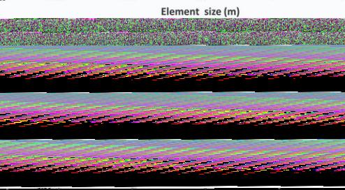
              The geometry of the model (i.e., dam
            
            
              with partial cut-off wall; k
            
            
              sat
            
            
              ,
            
            
              homogenous
            
            
              soil
            
            
              = 8.13×10
            
            
              -3
            
            
              m/day) analyzed is
            
            
              presented in Figure 1.
            
            
              In the reference article, convergence
            
            
              of the solution was obtained using a
            
            
              uniform mesh with an element size of
            
            
              0.5 m. From Figure 1 it can be seen
            
            
              that the converged solution obtained
            
            
              when using the automatic adaptive
            
            
              mesh refinement has larger elements
            
            
              in most parts of the analyzed domain.
            
            
              The exception is found around the
            
            
              cut-off wall where the element size is
            
            
              significantly smaller than the overall
            
            
              average element size. For the mesh
            
            
              presented in Figure 1, the calcu-
            
            
              lated flow rate was 6.82×10
            
            
              -7
            
            
              m
            
            
              3
            
            
              /s.
            
            
              Calculation time for the mesh pre-
            
            
              sented at Figure 1 was 0.01 minutes.
            
            
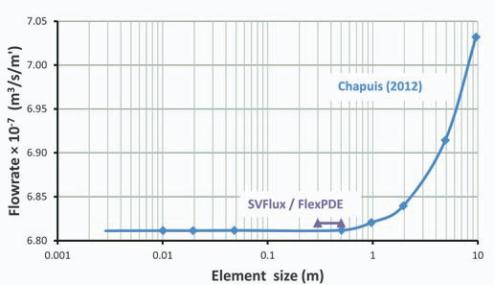
              Comparison of results obtained with
            
            
              manually-controlled meshes and
            
            
              automatic-controlled adaptive meshes
            
            
              are presented in Figure 2. Calculation
            
            
              computational times associated with
            
            
              using a disabled mesh generator with
            
            
              a specified maximum element size of
            
            
              0.5 m, increased to 7.37 minutes while
            
            
              the flow rate solution remained the
            
            
              same (note that an older computer was
            
            
              used for this study). The consequence
            
            
              of further reductions in the element
            
            
              size to 0.3 m was an increased calcula-
            
            
              tion time from 7.37 minutes to 36.03


                Figure 1. Partial cut-off wall model geometry with mesh


                generated using the automatic adaptive mesh generator.


                Figure 2. Converged leakage flow-rate for the cut-off


                example.