Basic HTML Version


www.geotechnicalnews.com
Geotechnical News • December 2012
39
GROUNDWATER
minutes while the flow rate remained
unchanged.
Confined aquifer example
The geometry of the second model
(i.e., pumping well in confined aqui-
fer; ksat, homogenous soil = 4.0×10⁻⁴
m/s ) is presented in Figure 3.
In the reference article (Chapuis,
2012) the solution converged using a
uniform mesh with an element size of
0.1 m. From Figure 3 it can be seen
that converged solution obtained with
use of the automatic adaptive mesh
has larger elements in most parts of
the analyzed domain, except around
the pumping well where the element
size is significantly smaller than the
overall average (0.2 m in average).
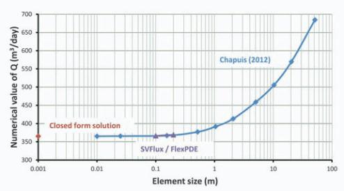
For the mesh presented in Figure 3 the
computed flow-rate was 369.17 m
3
/
day. The calculation time for the mesh
presented in Figure 3 was 0.02 min.
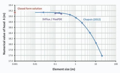
Comparison of flow-rate and total
head obtained when the mesh was
manually-controlled and when the
mesh was automatically generated
using an adaptive mesh generator is
presented in Fig-
ure 4 and Figure
5. Calculation
time for disabled
mesh generator
with a speci-
fied maximum
element size of
0.1 m (in the
region which
covers area from
pumping well to
the 20.15 m in the
radial direction), has increased to 1.15
minutes while the flow-rate solution
decreased to 366.54 m
3
/day. The size
of the elements in the remainder of the
domain was 1 m.
Conclusion
In the reference article author stated
that finer grid provides a more accu-
rate solution. However, the solutions
converged only after the mesh was
refined to an element size of 0.5 m (in
the cut-off example) and 0.1 m (in the
confined aquifer example), uniformly
distributed across the problem domain.
From Figure 1 and Figure 3 it can be
seen that mesh obtained when using
automatic adaptive mesh generators
can have much larger elements in
most parts of the domain while the
accuracy of the solution is preserved
as presented in Figure 2, Figure 4 and
Figure 5.
Chapuis (2012) suggested the creation
of a final confirmation/verification
mesh (i.e., a finer
mesh) to verify that solution has
actually converged (this is done to
define the true solution as accurately
as possible when closed-form solu-
tion is unknown). It was also stated
that this final verification step might
be a time consuming process (for long
transient problems computing time can
take hours or even days). For lengthy,
transient problems, it was suggested
that final verification mesh could be
omitted in order to save time. With use
of automatic adaptive mesh refine-
ment generators, this final verification
step is not necessary since the mesh
generator refines the mesh in various
parts of the domain until the solu-
tion converges within user specified
tolerance limits. Since the accuracy of
the solution depends on these toler-
ance limits, it is necessary that user
have a clear understanding of the finite
element method when using adaptive
mesh generators in an efficient man-
ner. It can’t be emphasized enough
that it is the engineer who must check
the numerical tools and their solutions.
However, is should be also noted that
for the default error limits should
result in a converged solution for
most standard geotechnical problems
defined in Eurocode 7 as Geotechnical
Category 1 and 2.
In summary, automatic an adaptive
mesh generator can also result in the
following benefits.
• A optimized (locally finer and lo-
cally coarser) mesh means fewer
number of equations,
Figure 3. Pumping well (confined aquifer) model geom-
etry with mesh generated by adaptive mesh generator;
take a note that few triangles have an angle higher than
90 degrees, which means a poor shape for calculations
(axisymmetric problem, radius of confined aquifer was
600 m).
Figure 4. Converged numerical flow-rates.
Figure 5. Converged total heads at r = 20.15 m.