Geotechnical News September 2011
35
GEO-INTEREST
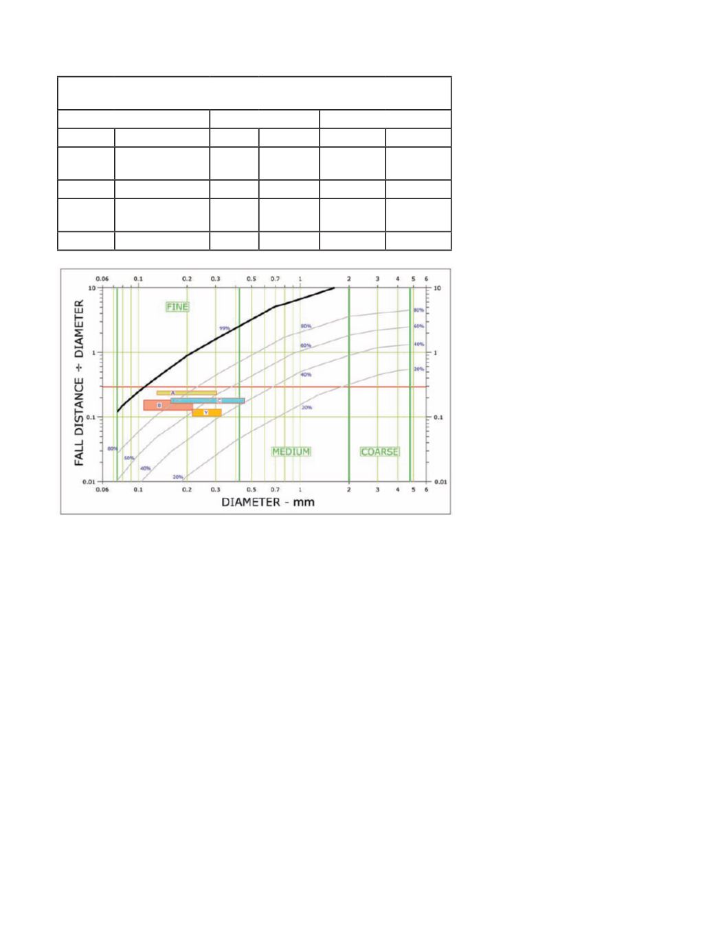
[F/D] in order to transfer 99% of its
buoyant weight to the water it is falling
through. Similarly the other percentage
labels are for lesser amounts of weight
transfer to the water.
The three rectangles, labeled A, B
and C are thus derived from Castro’s
three sets of triaxial tests over the range
of densities where the specimen lique-
fied under monotonic loading. The let-
ters are the same as those used by Cas-
tro in naming the three different sands
he used. The rectangle labeled “Y” is
for the extension tests which resulted in
liquefaction (steady state stress-strain)
of the Fraser River sand Vaid used.
The vertical sides of the rectangles
are at the D
85
and the D
15
gradation
sizes for each particular sand type.
The upper and lower horizontal sides
of the rectangles cover the range of
void ratios at which specimens were
made, and which resulted in liquefac-
tion failures. These values are listed in
the table, where it can be seen that soils
fall into the category of fine sands and
the equivalent F/D range lies between
0.1 and 0.25. Here it is necessary to
point out that although some of these
numbers are quite close to the red-line
value of 0.29, and might be consid-
ered as providing some support for this
proposal, this is not the case. Instead,
they need to be compared with the val-
ues along the black/grey curved lines
representing the percentage of weight
transfer to the water.
As may be seen from this mode of
presentation the losses in effective par-
ticle weight range from 40% to 90%
with the average being somewhat less
than we would expect during a lique-
faction failure. I believe a better inter-
pretation of this plot requires consider-
ation of the Crowding-factor [K], since
the % transfer lines are based on single
particle responses, whereas here we are
for the first time dealing with the soil
mass. “K”, which will be subsequently
introduced and developed in Part 5 of
this series, is essentially an amplifica-
tion factor on relative motion. As such
it has the effect of reducing the amount
of fall necessary to achieve a particular
level of weight transfer, and therefore,
should bring the curves more into line
with these laboratory results.
Shear Waves and Cyclic
Loading
Computer programs which deal with
the transmission of shear waves through
soil, such as SHAKE, have proven very
useful (and surprisingly accurate) in
predicting how tall buildings move/
sway about in response to earthquake
vibrations. These programs are based
on how small strains of different
frequencies would be either amplified
or attenuated as they pass through a
stable/intact soil-structure. I doubt if the
original authors would have condoned
their use for soils which were strained
to the extent that they were collapsing.
However that may be, what is known
for sure is that shear waves cannot
pass through a fluid, and this presents
a problem when dealing with soil we
expect to liquefy. Presumably that part
of the vulnerable deposit closest to the
excitation would be fluidized first. Then
the question arises as to how and why
would liquefaction trespass beyond
that boundary. Surely it couldn’t.
The complementary laboratory
testing, which involves cyclic load-
ing, I find equally difficult to accept
inasmuch as it bears on liquefaction.
Apart from believing that such testing
would have application only in the case
of shear wave transmission, the idea
of subjecting saturated sand inside a
sealed membrane to as many as a 1,000
stress reversals has always struck me as
some kind of abuse of specimen: For
some reason or other it makes me think
of those bad days in medieval times
when confessions were extracted by
torture.
As I visualize it, stress reversals
result in grain asperities been broken
off. These small pieces/dust are not
large enough to remain part of the
soil-structure. As a result the specimen
gradation tends to become gap-graded.
Table of Equivalent “Fall-to-Diameter” Ratio Limits
(values plotted as rectangles on Figure 11)
Sand Type
Size, mm
Fall ÷ Diameter
Symbol
Source
D85 D15
Upper
Lower
A
Salt Lake
earthfill
0.304 0.130
0.254
0.220
B
Ottawa Banding 0.217 0.108
0.183
0.127
C
Huachipato
Beach
0.452 0.159
0.197
0.163
Y
Fraser River
0.325 0.215
0.134
0.103
Figure 11. Castro and Vaid results on Fall/Diameter plot.


