30
Geotechnical News • June 2013
GROUNDWATER
to predict
n
e
. There are only curve
fitting methods. This is unfortunate for
consultants who simply assume some
n
e
value from their experience or the
literature, and use it with some pre-
dicted
α
L
. Further, if a field tracer test
is carried out, a theory may be chosen
and used to extract
n
e
by curve fitting.
The lack of research on
n
e
is regret-
table for those who have to protect
drinking water wells. Also, most field
breakthrough data are difficult to fit
with theoretical models (Fernandez-
Garcia et al. 2005; Pedretti and Fiori
2013). The theoretical study of tracer
tests has advanced but it has become
increasingly complex. Meanwhile,
consultants have to guess the field
n
e
and
α
L
values (most studies) or esti-
mate them by fitting the breakthrough
data to some model (a few studies).
The goal of this paper is to reduce
a gap between theoretical research
and practical needs. It makes use of
recently derived analytical equations
(Chapuis 2015) for the hydraulically
equivalent homogeneous aquifer
(HEHA), thus for
n
e
HEHA
and
α
L
HEHA
at field scale. The background is
briefly presented, and then, the predic-
tive equation for
n
e
is verified using
experimental data.
Background
Chapuis (2015) assumed that different
seepage velocities in stratified aquifers
create dispersion, which results in
large-scale values,
n
e
HEHA
and
α
L
HEHA
.
Two problems were examined and
solved. The first problem is rectilinear
seepage, at constant hydraulic gradi-
ent
i
, in a stratified horizontal confined
aquifer of constant thickness, where
K
varies only vertically. The second
problem is for a well pumping the
same aquifer at a constant flow rate
Q
, for radial steady-state seepage. The
perfect well is vertical and fully pen-
etrating. The radial groundwater flow
converges towards the well.
Initially the non-reactive tracer con-
centration
C
is zero everywhere. Start-
ing at time
t
= 0, the tracer enters the
external boundary at a concentration
C
0
(step function), which is main-
tained either forever or for a limited
time. It is assumed that small-scale
diffusion does not play a key role in
the flow and transport equations. Pure
convection is considered: the
C
0
step
function produces a piston flow in
each layer. The resulting analytical
equations for large-scale
n
e
HEHA
and
α
L
HEHA
are then derived. Variations at
the individual pore scale are not taken
into account.
Chapuis (2015) solved the two simple
problems first for a finite number of
layers, and for the HEHA having the
same flowrate for the same boundary
conditions, thus a single
K
value equal
to the averaged
K
ave
value. This is a
frequent assumption, but the assumed
homogeneity with
K
ave
is correct only
for the flowrate. Then, Chapuis (2015)
solved the two problems for a large
number of layers. Each layer No.
j
had
K
j
and
n
ej
values. The
K
j
values
followed a lognormal distribution of
mean
μ
ln
K
and variance
σ
2
ln
K
or they
follow a normal distribution of mean
μ
K
and variance
σ
2
K.
Moreover, the layers were assumed
to have parallel grain size distribu-
tions, with the same stress and strain
history, which yields local
nj
=
n
, and
n
ej
=
n
e
. The
theory (Chapuis
2015) makes no
assumption on
spatial correla-
tion. The water
seeps parallel
to stratification.
The velocity
field depends
upon the
K(z)
field, the constant
gradient
i
(at all
x
values for the
1
st
problem, at
any constant
r
value for the 2
nd
problem), and
n
ej
=
n
e
. The most conductive layer is
the first to supply tracer mass, and the
gradual input of all layers produces a
breakthrough curve (BTC).
For a lognormal
K
distribution,
Chapuis (2015) obtained a new solu-
tion that is close to the 1D solution
for the advective-dispersive equa-
tion (Ogata and Banks 1961). For the
HEHA,
n
e
HEHA
was obtained for
C/C
0
= 0.5 at time
t
50
ln
K
, which yielded
in which
K
50
is the value such as 50%
of the
K
values are lower than
K
50
.
Equation (1) confirms that
ne HEHA
is smaller than the single
n
e
of each
layer. It also confirms the frequently
observed “early” tracer arrival in field
tests. In general,
μ
ln
K
is between -11
and -7 (e.g., Chapuis 2013) whereas
σ
ln
K
is between 0 (spheres having the
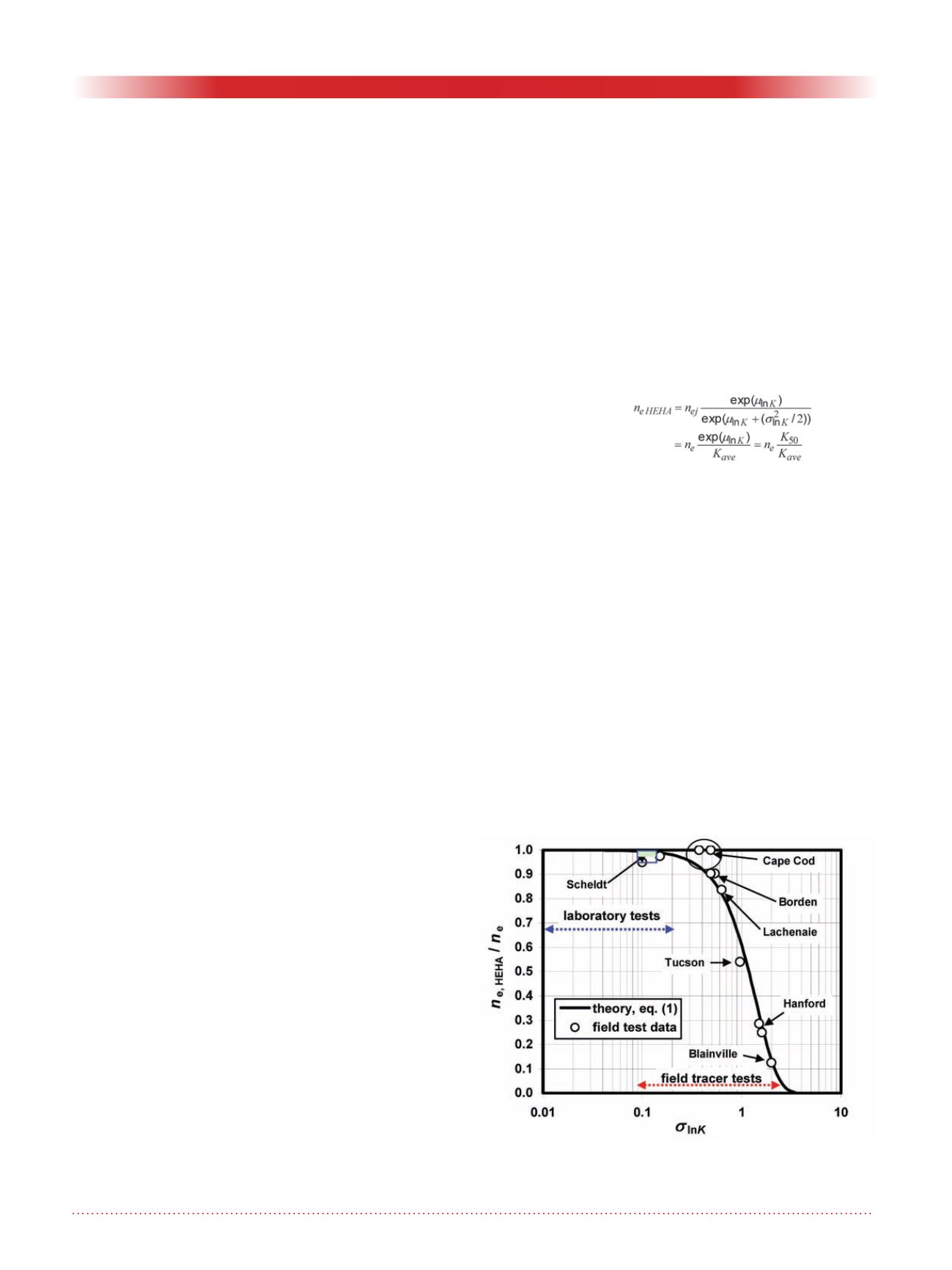
same diameter) and about 2. As a
result, Figure 1 shows how the ratio
(
n
e
HEHA
/ n
e
) varies in theory. Exam-
ples of tracer tests are given below to
verify eq. (1).
In the case of a normal
K
distribu-
tion, the theoretical development gave
(Chapuis 2015):
Figure 1. Variation of the ratio (n
e HEHA
/ n
ej
) predicted by
eq. (1) as a function of
μ
lnK
(from about -11 to -7) and
σ
lnK
(from about 0 to 2).
(1)


