32
Geotechnical News • June 2013
GROUNDWATER
0.9, which in retrospect justifies the
assumed equality.
The Borden test (Freyberg 1986;
Sudicky 1986) was carried out in
stratified sand of dry density
ρ
d
= 1.81
g/cm
3
, and specific gravity of solids,
G
s
= 2.71, which give
n
= 33.2%. The
test (Bales et al. 1997) gave
n
e
≈ 30%,
thus 90% of
n
(Mackay et al. 1986).
The variance of
ln
(
K
) was either 0.29
(Sudicky 1986) or 0.24 (Woodbury
and Sudicky 1991), which gave
σ
ln
K
=
0.54 or 0.49.
The Tucson test gave
n
e HEHA
≈ 0.5
n
(Stephens et al. 1998). The distribu-
tion
K
for the stratified aquifer was
given in Zhang and Brusseau (1998).
Ignoring the sub horizontal aquitard
lenses, it was found for this paper that
the aquifer sub layers (
K
≥ 10
-5
m/s)
yielded
σ
ln
K
= 0.96 (Chapuis 2016).
The Scheldt test was carried out in
uniform sand (with a few silt-clay
lenses) for which
n
≈ 0.39–0.40. The
K
values for the 14 layers forming the
aquifer were given in Vandenbohede
and Lebbe (2006). These were used
for this paper to draw a distribution
curve, which yielded
σ
ln
K
≈ 0.10–0.15.
The Hanford test was carried out in a
sand-and-gravel aquifer (Bierschenk
1959) and gave
n
e
= 0.10. The sub
layers had
n
values in the 0.35–0.40
range; the
K
values, between 3.5 x
10
-5
and 3.5 x 10
-2
m/s (Graham et al.
1981; Nevulis et al. 1989) were used
for this paper to draw the distribution
curve, which yielded
σ
ln
K
≈ 1.5–1.6.
Converging tracer tests were carried
out in a sand aquifer at Lachenaie
(Quebec) after steady-state seepage
was reached for a pumping test. The
tests yielded
n
e HEHA
= 33%, whereas
n
≈ 39–40%. More detail, includ-
ing the
K
distributions at small scale
(samples) and middle scale (slug tests
in monitoring wells) may be found in
Gloaguen et al. (2001) and Chapuis et
al. (2005). A lithium chloride solution
was injected as a spike in the short
screen of a monitoring well. Using
the grain size distributions and the
porosity, the small-scale
K
values were
predicted using the methods of Hazen-
Taylor (Hazen 1892; Taylor 1948; see
Chapuis 2004) and that of Chapuis
(2004). Each small scale
K
distribution
was fitted with lognormal and normal
functions, which correctly predicted
the large-scale
K
and
n
e HEHA
(Table 1).
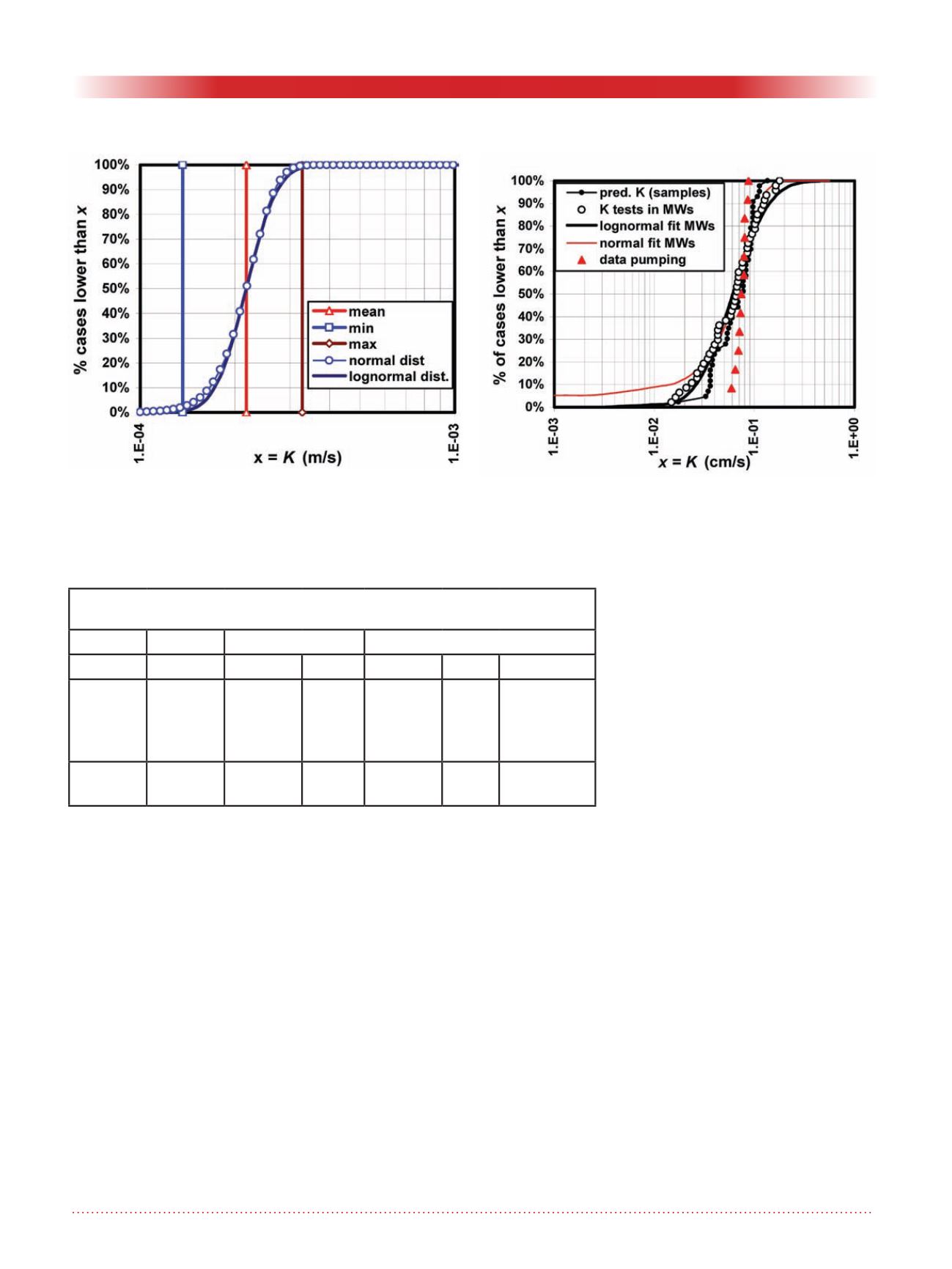
The middle-scale
K
values (slug tests)
were also adjusted with lognormal and
normal distributions (Fig. 3), which
gave the predicted large-scale
K
ave
and
n
e HEHA
. All results (Table 1) show
that the field
K
ave
and
n
e HEHA
are better
predicted by the lognormal
K
assump-
tion than by the normal
K
assumption.
However, the differences are small
Figure 2. Example of a laboratory tracer test: the K range
can be fitted with normal and lognormal K distributions,
which are very close.
Figure 3. Experimental K distributions for the Lachenaie
sand aquifer (Chapuis et al. 2005), with lognormal and
normal best fits for the slug tests in monitoring wells after
development.
Table 1. Lachenaie test: comparison of predicted and field values
for large-scale K and
n
eHEHA
Lognormal K dist.
Normal K distribution
Method scale
K
ave
(m/s)
n
eHEHA
K
ave
(m/s)
n
eHEHA
type
Hazen-
Taylor
Chapuis
Slug tests
small
small
middle
7.4 x 10
-4
7.5 x 10
-4
7.4 x 10
-4
0.312
0.318
0.324
7.0 x 10
-4
7.1 x 10
-4
6.5 x 10
-4
0.40
0.40
0.40
predicted
predicted
predicted
Pumping
Tracer
large
large
7.4 x 10
-4
-----------
-------
0.33
7.4 x 10
-4
-----------
-------
0.33
experimental
experimental


