34
Geotechnical News December 2010
Influence of Element Size in Numerical
Studies of Seepage:
Large-scale or Regional Studies
Robert P. Chapuis
Many of us use numerical codes to
study groundwater seepage within
aquifers and often to solve the
following inverse problem: What are
the values of the hydraulic conductivity
K
within an aquifer given the hydraulic
heads at some monitoring wells, and
some (usually limited) information
about flow rates, pumping and field
permeability test data? Textbooks
teach us that an inverse problem can
have several solutions. For example,
a numerical code that correctly solves
the inverse problem on a given grid
may yield an incorrect solution on a
more refined grid. The key questions
are: why does this happen, and how can
we control this?
A Simple Example Problem
A simple example will illustrate what
happens numerically with different
grids. We examine an ideal confined
aquifer, which is homogenous and
horizontal, with constant thickness
and constant saturated hydraulic
conductivity. The hydraulic gradient
is constant in the aquifer before any
pumping. The well is pumped at a
constant rate and has reached steady-
state conditions.
The finite element code Seep/W
(Geo-slope International 2003), which
has passed a battery of tests (Chapuis
et al. 2001), is used here. This code
uses the soil characteristic functions,
K
(
u
w
) and
θ
(
u
w
), in which
u
w
is the pore
water pressure,
K
(
u
w
) is the hydraulic
conductivity function, and
θ
(
u
w
) is the
volumetric water content function. The
equations of Darcy (1856) for seep-
age, and Richards (1931) for fluid mass
conservation, are solved numerically
as
u
w
-based equations. The code can
find complete solutions for saturated
and unsaturated seepage. Once the nu-
merical analysis is completed, the code
provides equipotentials, flow lines and
flow rates through previously defined
surfaces.
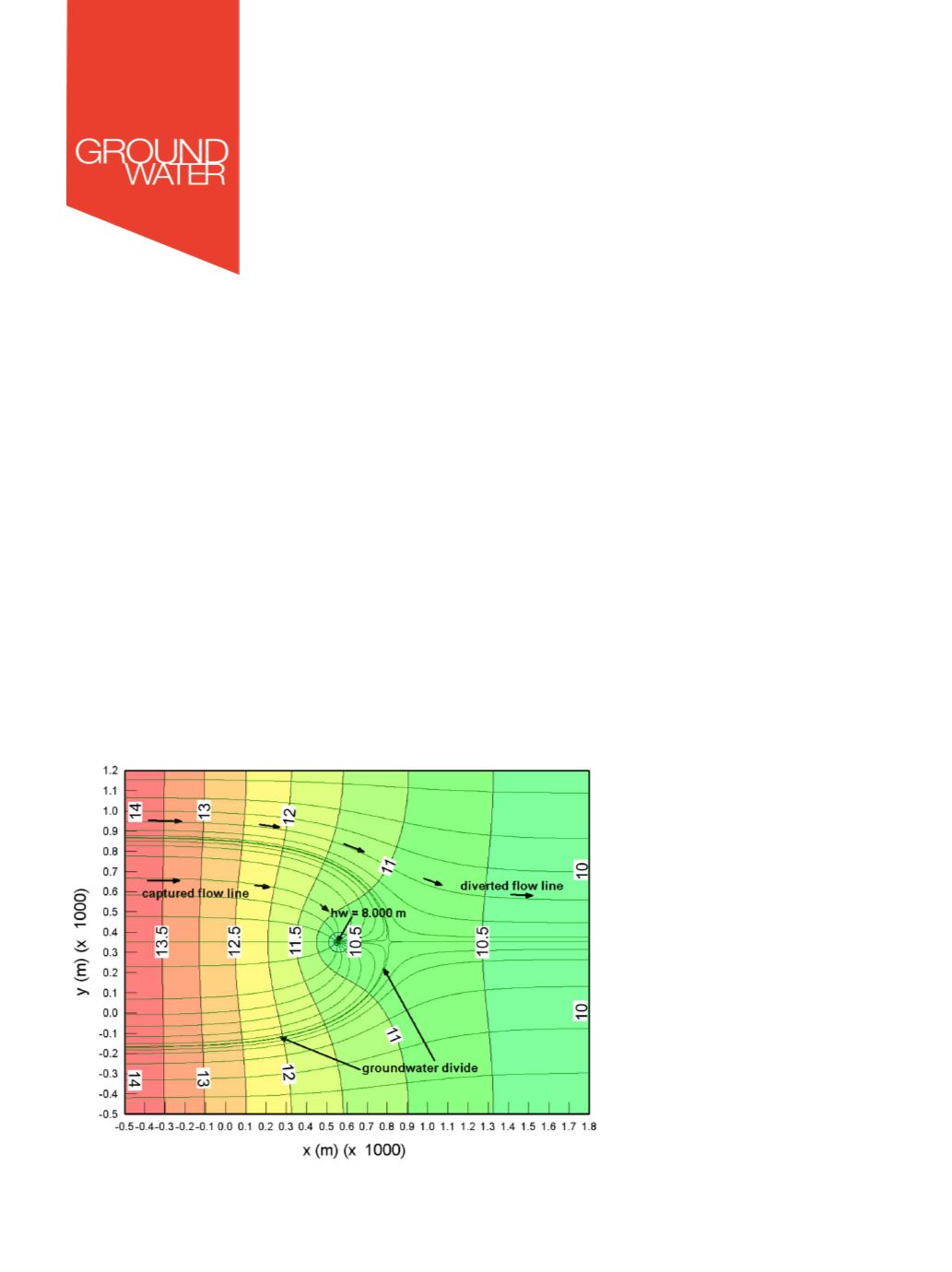
We study the steady-state pumping
problem in a rectangular ideal confined
aquifer (Figure 1). The aquifer abscissa
x
varies from -500 m to +1800 m. The
aquifer ordinate
y
varies from -500 m
to +1200 m. The aquifer transmissiv-
ity (
T = Kb
= 4 x 10
-4
m
2
/s) and thick-
ness
b
are constant. The pumping well
is located at
x
= 550 m,
y
= 350 m. The
boundary conditions (BC) for all grids
are as follows: impervious boundary
(or flow line) along the lateral bound-
aries
y
= -500 m and
y
= +1200 m; con-
stant hydraulic head
h
= 14.00 m along
the upgradient boundary
x
= -500 m;
constant hydraulic head
h
= 10.00 m
Figure 1. Example flownet for the ideal confined aquifer, steady-state pumping
(equipotentials in metres).


