Geotechnical News December 2010
35
GROUNDWATER
along the downgradient boundary
x
=
+1800 m. Thus, before pumping the
regional gradient is constant at 1.7391
x
10
-3
(4 m / 2300 m) in the ideal aqui-
fer. A flownet with the pumping well is
shown in Figure 1 for one of the seven
grids that have been considered for this
paper. At the pumping well, the bound-
ary condition (BC) is either a constant
head
h
w
of 8.00 m (corresponding to a
drawdown of 4.174 m) or a constant
flow rate
Q
w
of 87 m
3
/d. These two BC
conditions are our “observations” at
the pumping well. Using several grids
we have found what is the computed
flowrate when
h
w
= 8 m is used as the
BC condition, and what is the
h
w
value
when Q = 87 m
3
/d is used as the BC
condition. Then, we have found for
each grid what is the
K
value to be used
to match both the
h
w
and Q “observed”
values.
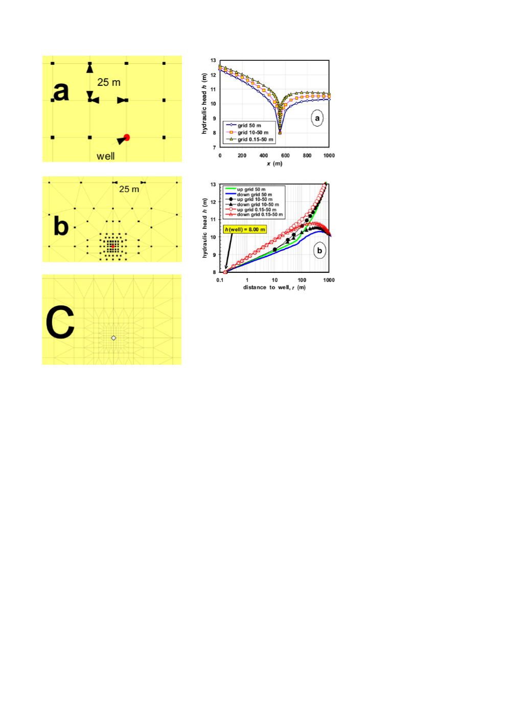
Seven grids were used to study how
the element size influences the numeri-
cal solution. Square elements of 100,
50, or 25 m (Figure 2a) were used for
grids 1 to 3. The pumping well of grid 1
is the center of a 100 m square element
divided into 4 triangles. Grids 3 to 6
have uniform meshes of 50 m except
in the 200 m x 200 m square around
the well: their smallest elements have
a size of 10, 2.5 and 1.0 m (Figure 2b).
For grids 1 to 6, the well is simply rep-
resented by a single node at the well
center. Grid 7 has smallest elements of
15 cm around the well to better simu-
late a real well of diameter 30 cm; the
well screen is represented by the 4
nodes of a square (Figure 2c), which is
a rough but still reasonable representa-
tion of a cylindrical vertical well.
Numerical Results
a. Using the well drawdown as the
boundary condition
A few numerical results are shown in
Figures 3 and 4. It is observed first
that the coarser the grid, the wider the
drawdown cone (Figure 3a). The local
variation of hydraulic head
h
(and
therefore the gradient) close to the
well is poorly estimated using grids
with equal square elements (Figure
3b). To correctly compute the gradient,
and thus the pumped flow rate, a very
refined mesh is needed.
When a node (or vertical line of
nodes) represents the pumping well,
the numerical code gives an incorrect
gradient in the elements containing the
well node(s). Specifying a drawdown
at a well node creates a gradient pass-
ing from a positive to a negative value
at the well node, thus a discontinuity
which results in poor numerical esti-
mates of both gradient and flow rate.
The pumped flow rate,
Q
, for the
same drawdown at the well, increases
with the element size of the grid (Fig-
ure 4). With equal square elements of
100 m, the
Q
value is overestimated by
94% in this problem. The refined (6
th
)
grid, with elements of 1.0 m close to
the well, provided a
Q
value 8% higher
than that of the most refined 7
th
grid.
b. Using the pumped flow rate as the
boundary condition
When the pumped flow rate (87 m
3
/d)
is used as the BC at the pumped well,
then the computed hydraulic head at
the well of grids 1 to 6 is not 8.00 m as
it should be to match the observation.
Therefore, in order to match the
observed
Q
and
h
w
at the pumping well,
the aquifer
K
value must be modified as
shown in Figure 5. With equal square
elements of 100 m, the computer best
fit
K
value is only 51% of the true
K
value. As previously seen for the
Q
value, only grid 7 provides a correct
best fit estimate of the
K
value.
Our results for the simple case of
an ideal confined aquifer (Figures 3 to
5) indicate that the best fit with coarse
grids yield poor estimates of either the
K
values or the
Q
values. If the draw-
down data and measured
Q
data are
used as benchmarks to solve the inverse
problem, then all values of
K
providing
a best fit will be severely underesti-
mated. This means that the water and
contaminant transport velocities will
Figure 2. Three examples of grids that
have been used to study groundwa-
ter steady-state seepage in the ideal
confined aquifer: (a) uniform grid,
the pumping well is represented by a
single node; (b) refined grid around
the pumping well, still represented by
a single node; (c) very refined grid
(squares of 15 cm) around the pumping
well, represented by four nodes.
Figure 3. Numerical results in the x di-
rection for several grids. The BC at the
pumping well is h = 8.00. (a) Hydrau-
lic head versus x; (b) Hydraulic head
versus r along the x-axis.


