36
Geotechnical News December 2010
GROUNDWATER
be underestimated by a factor that may
be close to 2 in the present numerical
study. Only the grids with very refined
meshes around the pumping wells can
provide correct estimates for the values
of
K
and Darcy velocities.
Consequences for the General
Inverse Problem
Consider now briefly the more
general inverse problem of finding the
distribution of the
K
values within an
aquifer knowing a few hydraulic head
data at a few monitoring wells, and a
few flow rates and drawdown data at
a few pumping wells. Coarse regular
grids are used most of the time to solve
this inverse problem.
To understand why coarse grids are
used, consider a 40 m thick unconfined
aquifer over a surface of 7 km x 10 km.
The numerical model may include 40
layers for the unconfined aquifer, thus
40 elements in the vertical direction. In
the horizontal plane, if the model uses
square elements of side 50 m, there will
be 140 x 200 elements. In the volume,
there will thus a total of 40 x 140 x
200 = 1,232,000 elements. Few codes
can solve the equations for such a high
number of elements, but the grid is still
coarse. If the unconfined aquifer is lo-
cated above a confined aquifer, water
will be exchanged between the aquifers
through an aquitard. The volumes of
exchanged water cannot be neglected
for such a large scale problem. The
study of the regional system may need
20 more layers for the aquitard and the
deeper aquifer, which will increase the
number of elements up to 1,848,000.
Using coarse grids to study regional
problems has two major drawbacks
from the point of view of numerical
analysis: (1) excessive element di-
mensions and (2) excessive aspect
ratios. The element aspect ratio is the
ratio of its maximum dimension to its
minimum dimension, 50 in the above
example. To avoid inaccuracies, the as-
pect ratio should be kept close to one,
but can reach 2 or 3 to accommodate
geometric constraints, as used in some
textbooks of numerical analysis.
The consequences of the first major
deficiency have been shown in Figures
3-4-5 for our simple 2D example: us-
ing large elements creates large errors,
even if the aspect ratio for the seven
grids of our example did not exceed
2. This occurs because a coarse grid
cannot provide a correct solution to an
inverse problem with pumping wells,
due to the discontinuity in hydraulic
gradient at each well, a mathemati-
cal singularity in the mesh, which is
poorly treated by any numerical code.
Even when the code’s solution meth-
ods are unknown, the errors and con-
vergence characteristics can be studied
using several theories and techniques
(Roache 1994, 2009). The related
mathematical issues, however, are be-
yond the scope of this short paper.
The second major deficiency is due
to excessive aspect ratios. In the pre-
ceding 3D regional example, the aspect
ratio is 50, whereas it is recommended
to keep it below 2 or 3. This high value
of the aspect ratio generates more error
in a 3D regional study than that previ-
ously found for our 2D ideal case study
(with an aspect ratio below 2).
In addition to these two major de-
ficiencies, the results obtained with a
coarse 3D grid may also be plagued
by errors resulting from cumulative
round-off errors: this increases with the
number of elements and depends on the
accuracy with which numbers are ma-
nipulated in the computer.
According to our experience, most
of the time, numerical studies are made
without addressing grid adequacy and
convergence issues. Due to current
limitations of computers, large grids
seem necessary to study regional prob-
lems. However, consultants and their
clients should be aware that large grids
are prone to provide incorrect answers
to inverse problems.
General Rules for Meshing
Over the past few decades, more
advanced computer methods have
become available: they frequently
give an illusion of being easy to use.
We have just seen that these numerical
tools are still complex to handle. In
the 1980’s and 1990’s the number of
nodes was a key parameter because the
computer memory was limited and the
computers were relatively slow. Since
the computing time for a given problem
is roughly proportional to the square or
the cube of the number of nodes, there
was a tendency to use simple meshes
and thus limit the number of nodes.
With the present computer capacity,
there seems to be less concern for the
number of nodes. This does not mean,
however, that we should always model
very finely any problem.
A few basic principles should be
observed, which are provided below.
First, we must have a preliminary idea
of how the hydraulic head varies with-
in the volume of our study. For a first
appraisal we can use a coarse mesh,
which will give us a first solution. We
must examine this first solution and
identify the zones with large local
variations in hydraulic head
h
, and (for
unsaturated zones) in water pressure
u
.
These zones are those where our mesh
must be refined. For a second apprais-
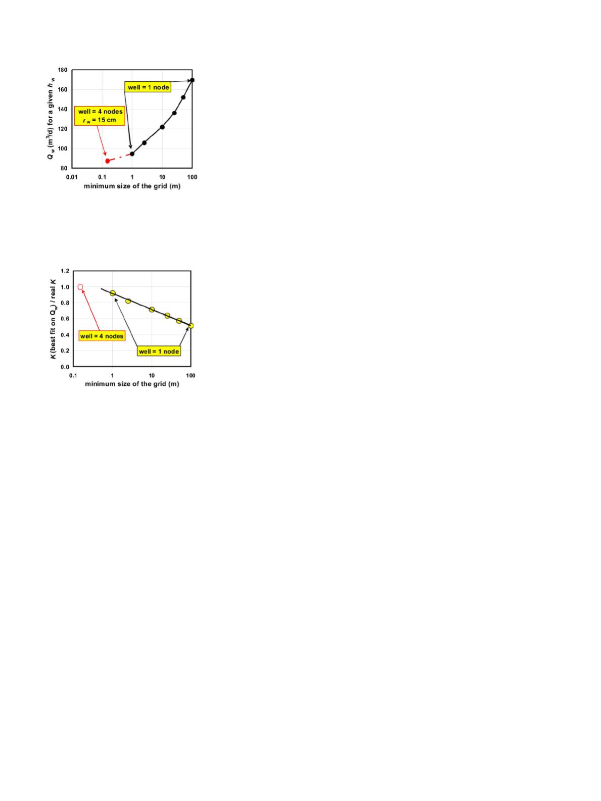
Figure 4. Numerical results for the
pumped flow rate when the same draw-
down is the boundary condition at the
pumping well, the grid size being the
only variable in the studied problem.
Figure 5. Numerical results when the
same flow rate is the boundary condi-
tion at the pumping well, the grid size
being the only variable in the studied
problem: values of the required hy-
draulic conductivity (or transmissivity)
to be used for the ideal aquifer.


