32
Geotechnical News • September 2012
GROUNDWATER
initial mesh of the regional study, it
will increase to 7.5 to 30 days, which
may be impractical. This explains why
numerical studies of regional seepage
may yield poor solutions, especially
for unconfined aquifers (Chapuis
2010).
Example and numerical results
Our example here is that of a 10
m high vertical column. This is a
1D (one-dimensional) steady-state
problem. The
boundary condi-
tions (BCs) are
as follows: the
BC at
z
= 0 m is
h
= 0 m; the BC
at
z
= 10 m is a
Darcy velocity
of 2 x 10
-8
m/s
(imposed flow
rate); the side
of the column is
impervious.
Eight meshes
with a single ele-
ment height were
used to study
how the element
size influences
the numerical
solution: the
element sizes are
100, 50, 25, 10, 5, 2, 1, and 0.1 cm.
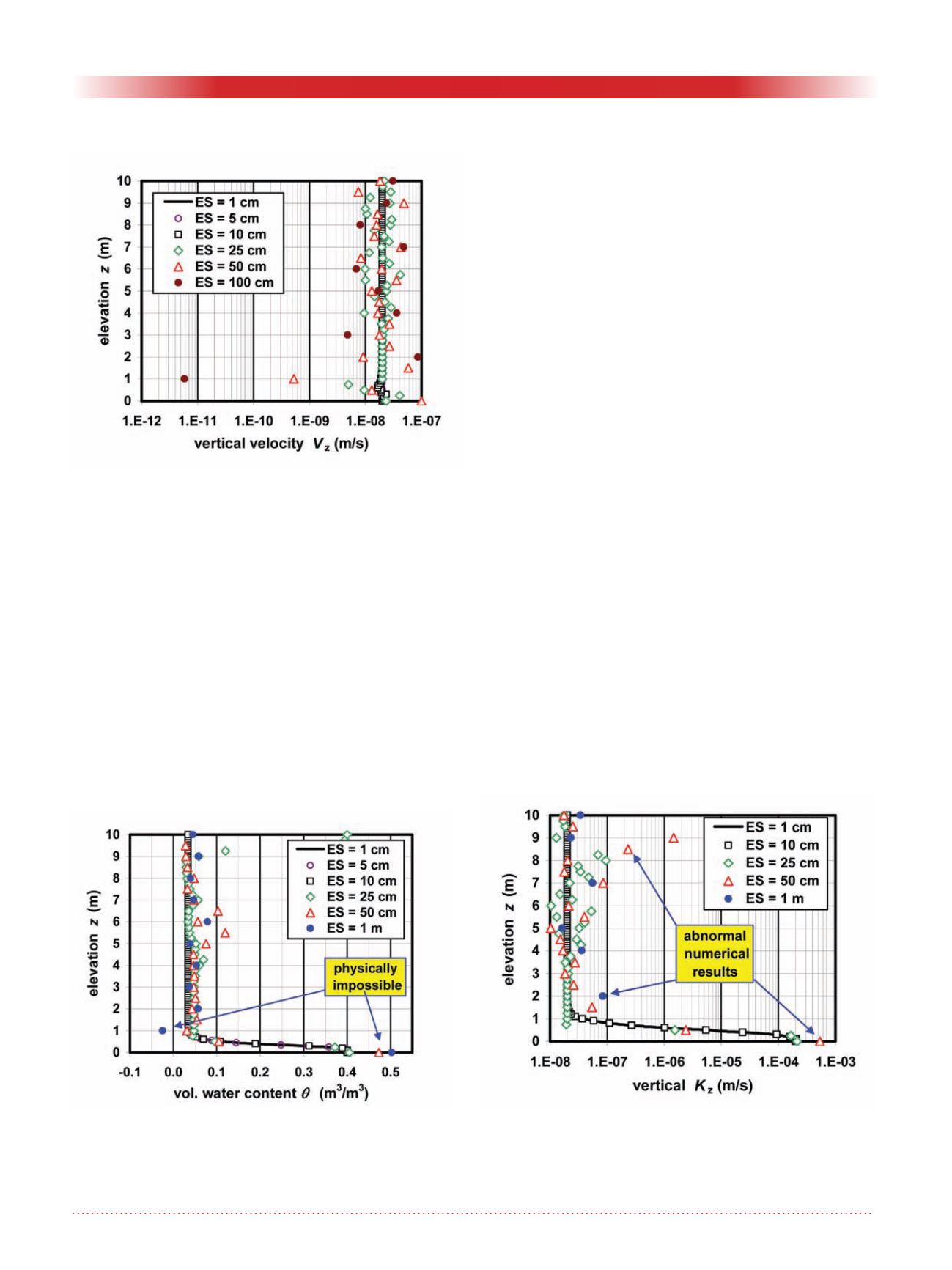
A few numerical results are given in
Figures 2-6. It is observed first that
coarse meshes provide a poor evalu-
ation of
h
versus elevation
z
(Fig. 2),
with numerical oscillations around the
correct
h
value obtained using 1cm (or
less) high elements.
The numerical error on a single
h
value, for example
h
(
z
= 1 m), is about 200% with ele-
ments of 25 cm; it becomes less than
3% when the element size is smaller
than 10 cm. Other error values (larger
or smaller) can be found for the h
value at other elevations
z
. For larger
elements, the error is random or oscil-
lating. For smaller elements, the error
smoothly follows the characteristics
of the interpolation scheme (Fig. 3).
When the algorithms used in a code
are known, the errors and convergence
characteristics of the finite element
equations can be studied mathemati-
cally. This is, however, outside the
scope of this short paper.
The element size influences the
numerically calculated vertical
velocity,
V
z
, which involves the local
gradient (
dh/dz
) and the local unsatu-
rated
K
value. However, the problem
definition implies mathematically that
V
z
has a constant value in the column.
The numerical solutions have large
fluctuations for element sizes between
100 and 25 cm, and small fluctuations
of about ± 15% at the bottom of the
column for a 10-cm element size (Fig.
4). The previously proposed rule-of-
thumb – restrict the element height to
the value giving a maximum change of
one order of magnitude for
K
in a no-
Figure 4. The element size has a large influence on V
z
.
However, the problem definition implies that in the real
solution V
z
is constant.
Figure 5. Solutions having converged numerically: The
values for
θ
oscillate when large elements are used, and
can take physically impossible values, either negative or
higher than the value at saturation.
Figure 6. Solutions having converged numerically: The
values for K oscillate when large elements are used, and
can take a value higher than the saturated one.


