Geotechnical News June 2011
49
GEO-INTEREST
component F
B
is a reasonable thing to
do for R
e
values up to about 1.
The blue line marked “P” running
along the C
D
= 1 ordinate in this fig-
ure corresponds to assuming F
D
could
be replaced by the Pressure component
equation, F
P
, that is assuming F
D
= F
P
.
It is obvious that this effort at replica-
tion leads to gross underestimations
until it cuts the C
D
curve at about R
e
= 100. Beyond this point it produces
equivalent C
D
values which are an
overestimation by a factor of about 2.
Therefore, the adoption of neither
analogy on which these lines are based
is acceptable in its own right for the full
range of C
D
of interest to us.
A purple line (with open circles)
“B+P” shows the result of the simple
addition of the ordinates of lines B
and P: This is equivalent to assuming
that the effects of both the Bearing and
Pressure components act simultane-
ously on the particle. By this means the
departure from the experimental curve
is reduced considerably, to an amount
which, in the context of a parameter
which has a practical variability of
seven orders of magnitude, might be
considered a reasonably approxima-
tion. Nevertheless, because I want to
bring the combined influences of the
two components (F
B
and F
P
) into full
alignment with Rouse’s C
D
over the
full range of R
e
it became necessary to
introduce and apply a correction factor.
This is the “L–factor”.
In applying an alignment factor to
the two separate and additive compo-
nents of Drag there is a choice. With-
out resulting in any inaccuracy to the
value of the Drag Force F
D
computed,
a non-dimensional L-factor can either
be applied as an overall multiplier,
as in L (F
B
+ F
P
), or as a component-
specific multiplier, as in (F
B
+ L F
P
). At
this stage of the development it is more
instructive to use the latter alternative,
and so, in Figure 8 the appropriate val-
ues of the L-factor are plotted for use in
the equation:
F
D
= F
B
+ L F
P
Across the range of interest to us the
values of the L-factor vary between 0.0
and 2.9. Here then are the sort of num-
bers I can keep in my head, something I
could never do with C
D
, the equivalent
values of which vary between 0.39 and
3,350,000 over the same domain.
You will see “soil-type” labels
marked across the R
e
range in Figure 8.
It is necessary to say that these labels
apply only at Terminal Velocity. But
because up till now we have concerned
ourselves mainly with the liquefaction
phenomenon I have added them to help
put thing into some context.
Modifying Mechanics – From
Fluid to Soil
At this stage we can now rewrite the
hydraulics style formula for Drag
Force, F
D
= C
D
ρAv
2
/2, in geotechnical
terms as follows:
F
D
= F
B
+ L F
P
where: F
B
= q
ult
A
F
P
= γ
w
h A
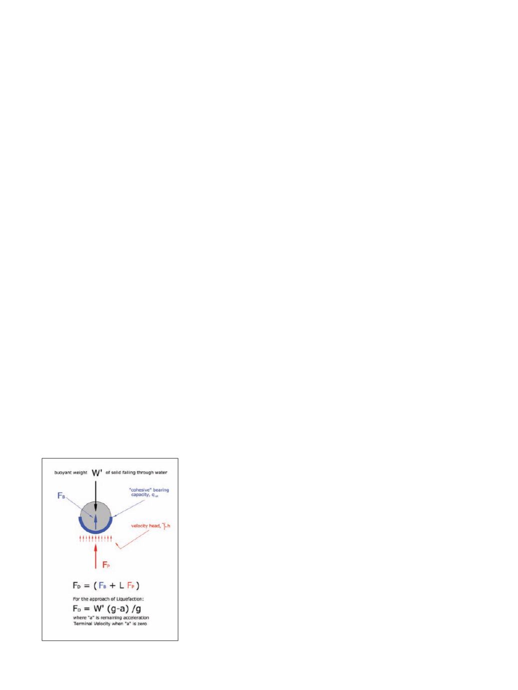
I’ve drawn the free-body diagram in
Figure 9 to help illustrate the balance
of forces involved in this approach.
This shows the formulation for the spe-
cial case of liquefaction. Later in this
series of articles the more general case
of soil-structure deformation will be il-
lustrated.
This geotechnical version, which
gives exactly the same answers as the
original, allows contemplation of sol-
id-to-water interaction in terms of two
separate mechanisms with which we
are quite familiar ourselves. And now
we are free to think of fine particles as
gradually settling footings, and to think
of gravel as solid impediments con-
fronting the impulse of flowing water.
But there is more to the above than
just appropriation of the good work
of our hydraulics colleagues. What
we might now have at our disposal is
a two-part elemental vector pointing
along a potential gradient parallel with
the thrust of soil-structure distortion.
This comes about because the force F
D
cited above is generated by each indi-
vidual particle in that part of the satu-
rated mass which is being moved. It
is quite similar to a seepage gradient
where water moves through soil under
the influence of an external hydraulic
gradient. The difference is that in the
case of steady state seepage there is
no instability or geometric alteration
of the soil-structure, whereas what we
are dealing with in these articles is pore
pressure change brought about by a de-
forming soil-structures.
In practical terms I find it interesting
that for relative velocities around those
associated with liquefaction, the L-
factor has the following values: across
the full silt size range L equals zero; it
reaches a peak for fine sands; and then
falls to around 0.5 for gravels where
turbulent flows are to be expected.
It is a consequence of how the Bear-
ing component was formulated that it
may be concluded that the term F
B
is not
a contributor to pore pressure. Herein,
the energy derived from the work done
as the Drag Force progresses may be
spent entirely in overcoming viscos-
ity, or following the analogy adopted
here, “cohesion” and, I suppose, just
dissipated as entropy/heat. Similarly,
it is consistent to presume that it is only
the Pressure component F
P
which con-
tributes to pore water pressurization,
and this takes place as kinetic energy
is converted to static potential on the
upstream side of solids confronting the
water’s relative velocity. Following
this line of reasoning we will proceed
from here on the understanding that all
to do with excess pore water pressure
in soils under deformation is contained
in the term F
P
, and that F
B
is a thing
apart.
Figure 9. Forces on falling ball.


