34
Geotechnical News • March 2012
GROUNDWATER
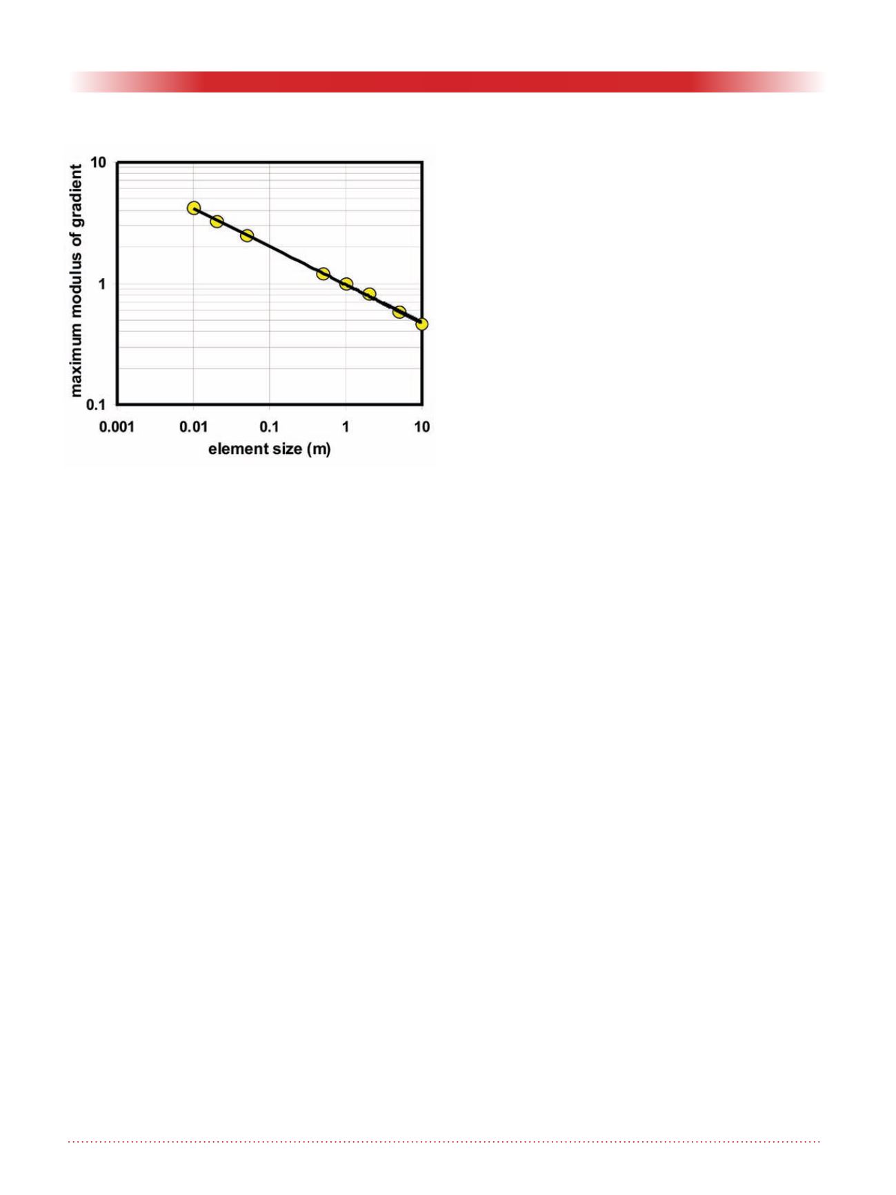
(Figure 5) but the relative error is still
about 7% for elements of 1 m. The
error drops to about 1% for elements
of 20 cm and about 0.1% for elements
of 5 cm. Similarly, the numerical value
for
h
(
r
= 20.15 m) converges towards
the closed-form solution (Figure 6),
but elements of 10 cm or less are
needed for a good accuracy.
For this example, note that the 2003
version of the code has a marked
advantage over the 2007 version,
because it can use a progressive
(logarithmic) meshing, which has
been removed in the 2007 version
that uses a different meshing process.
The logarithmic meshing provides
a much better accuracy for a much
smaller number of elements (Figure
7), which reduces the calculation time,
especially for transient problems. It
enables the use of very small elements
close to the screen, where the gradient
reaches its maximum, and large ele-
ments at the distant boundary, the size
of elements increasing gradually as the
radial distance increases.
General rules for meshing
As for large-scale groundwater stud-
ies, a few basic principles should
be observed for adequately treating
small-scale
details in numeri-
cal studies. First,
we must have
a preliminary
idea of how the
hydraulic head
varies within
the volume of
our study. For a
first appraisal we
can use a coarse
mesh, which
will give us a
first solution. We
must examine
this first solution
and identify the
zones with large
local variations
in hydraulic
head
h
, and (for
unsaturated zones) in water pressure
u
. These zones are those where our
mesh must be refined. For a second
appraisal, we can keep the large initial
mesh for the volumes where the
h
variations are small, and generate
finer meshes in the volumes of high
h
variations (high gradient zones).
When examining the second solution
and the zones of high variations, we
may find that some local refinements
are still needed. Once we are satisfied
with our last refinement and believe
that further refinement would add
nothing, we should not be satisfied
with our belief, but must prove it. We
must prepare a confirmation mesh in
which all elements will be smaller (by
half, for example) of what we thought
would be our last mesh. The confir-
mation mesh should give the same
results (heads, gradients, velocities,
flow rates, etc.) as our last mesh. If so,
then we have the proof that we have
designed and retained a correct mesh.
Note that the computing time for the
verification mesh may be about four
to nine times longer than the time for
our final and correct mesh. Thus, we
should avoid using the verification
mesh for long transient problems (the
computing time for this verification
could take many hours or even days)
but use it first for faster-to-solve
steady-state problems (which could
then also serve as initial conditions for
the longer transient simulations).
Two simple rules to observe are:
(i) The higher the local variations in
h
(anywhere), gradient (anywhere)
and u
w
(unsaturated zones), the fin-
er the local mesh;
(ii) The final solution must be
independent of the mesh size.
Conclusion
This short paper has examined two
examples, a partial cut-off wall for a
dam, and a steady state pumping test
of a confined aquifer. For the two
examples, the code used here reached
immediate numerical convergence
in two steps, the relative error on the
modulus of the pore pressure vector
being less than 10
-6
. This rapid con-
vergence is mostly due to the linear-
ity of equations for fully saturated
seepage and steady state. However,
different numerical solutions were
obtained for different grid sizes. In
short, we observed that the finer the
grid, the more accurate the numerical
solution. It is also important to model
all geometric details as accurately as
possible. In areas where the gradient
reaches a local maximum or mini-
mum, the use of progressive or loga-
rithmic meshing was shown to provide
a clear advantage in terms of accuracy
and calculation time.
To complement this paper which
focuses on small scale details with
high local variations of the hydraulic
head and gradient, and the previ-
ous paper on large-scale studies, a
forthcoming paper will provide a few
examples for cases in which unsatu-
rated seepage plays a key role.
References
Chapuis, R.P. 2009. Relating hydraulic
gradient, quicksand, bottom heave,
and internal erosion of fine par-
ticles. Geotechnical News, 27(4):
36–38.
Figure 4. Partial cut-off wall: Divergence of the local max-
imum gradient at the upstream of the cut-off wall toe.


